Assesses the model's calibration quality with the help of the pairwise complete modelled as well as observed loads and the following metrics:
NSE: Nash-Sutcliffe Efficiency
mNSE: Modified Nash-Sutcliffe Efficiency (
j = 1)KGE: Modified Kling-Gupta Efficiency
RMSE: Root Mean Square Error
PBIAS: Percent Bias
RSR: Ratio of the RMSE to the standard deviation of the observations
RCV: Ratio of the coefficients of variation
GMRAE: Geometric Mean Relative Absolute Error
MdRAE: Median Relative Absolute Error
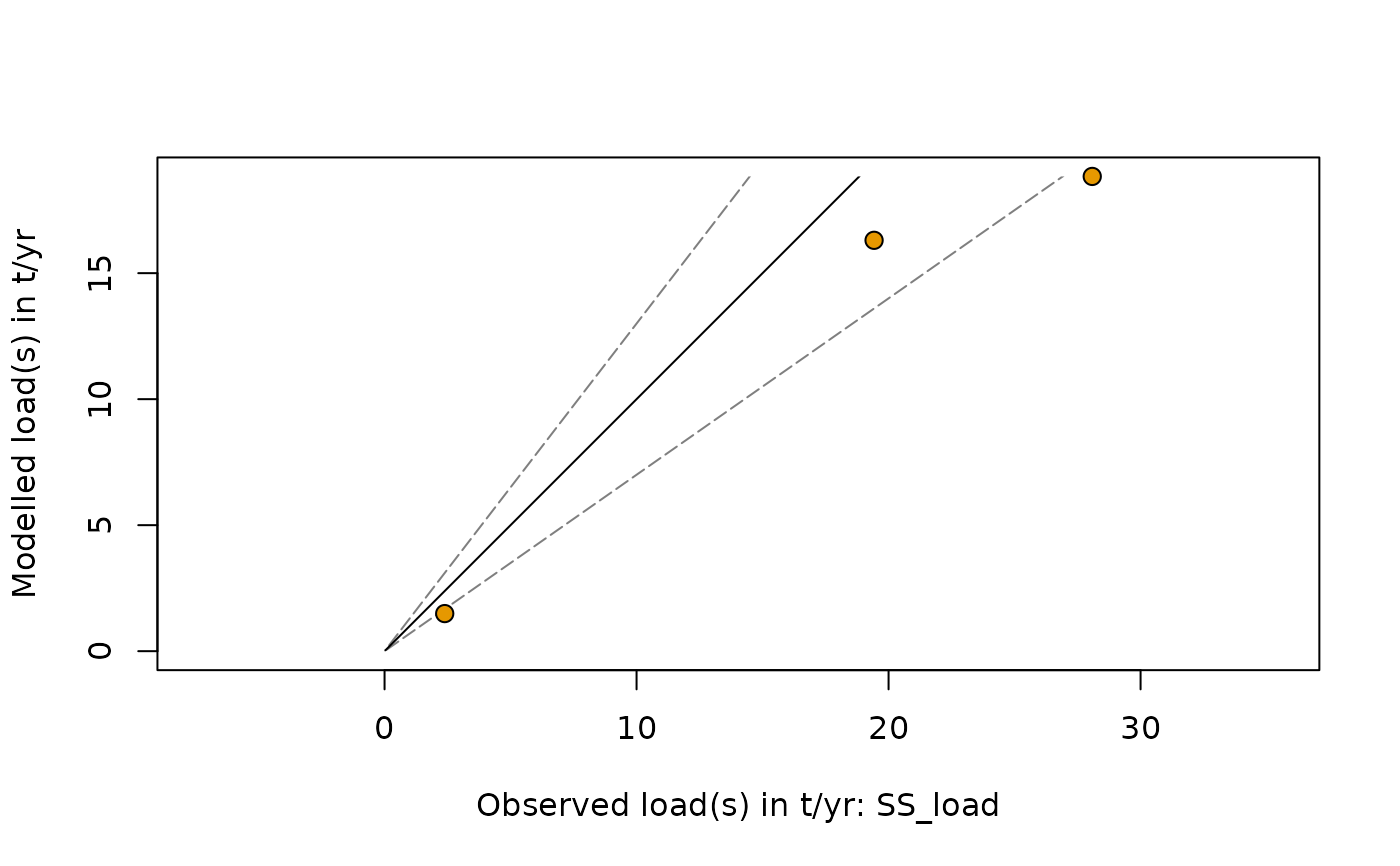
In addition, a scatter plot with the observed river loads on the x- and the modelled river loads on the y-axis is displayed and provides a visual impression of the model performance. Other elements of this plot are an identity line (solid) and plus/minus 30% deviation lines (dashed).
# S4 method for class 'RPhosFate'
calibrationQuality(x, substance, col)
Arguments
- x
An S4
RPhosFateriver catchment object.- substance
A character string specifying the substance to calculate.
- col
A character string specifying the calibration data column with the respective substance river loads.
Value
A named numeric vector containing the assessed metrics along with the in-channel retention ratio (one minus sum of xxt at catchment outlet(s) divided by sum of xxt_inp).
References
Nash, J.E., Sutcliffe, J.V., 1970. River flow forecasting through conceptual models part I – a discussion of principles. Journal of Hydrology 10, 282–290. https://doi.org/10.1016/0022-1694(70)90255-6
Legates, D.R., McCabe Jr., G.J., 1999. Evaluating the use of “goodness-of-fit” measures in hydrologic and hydroclimatic model validation. Water Resources Research 35, 233–241. https://doi.org/10.1029/1998WR900018
Kling, H., Fuchs, M., Paulin, M., 2012. Runoff conditions in the upper Danube basin under an ensemble of climate change scenarios. Journal of Hydrology 424–425, 264–277. https://doi.org/10.1016/j.jhydrol.2012.01.011
Moriasi, D.N., Arnold, J.G., Van Liew, M.W., Bingner, R.L., Harmel, R.D., Veith, T.L., 2007. Model evaluation guidelines for systematic quantification of accuracy in watershed simulations. Transactions of the ASABE 50, 885–900.
See also
Examples
# \donttest{
# temporary demonstration project copy
cv_dir <- demoProject()
#> Warning: A folder called "demoProject" already exists and is left as is.
# load temporary demonstration project
x <- RPhosFate(
  cv_dir = cv_dir,
  ls_ini = TRUE
)
# presupposed method calls
x <- firstRun(x, "SS")
x <- snapGauges(x)

calibrationQuality(x, "SS", "SS_load")# }
#> NSE:   0.6071161
#> mNSE:  0.4420663
#> KGE:   0.6753664
#> RMSE:  6.690713
#> PBIAS: -31.9
#> RSR:   0.5117838
#> RCV:   0.9389487
#> GMRAE: 0.3970503
#> MdRAE: 0.9200186
#>
#> In-channel retention ratio: -2.220446e-16
#>